Interpreting interaction coefficient in R (Part1 lm) UPDATED

(going through this post again three years after I posted it. Made some, hopefully useful, changes)

(01.2018: further changes following DT comment)

Interaction are the funny interesting part of ecology, the most fun during data analysis is when you try to understand and to derive explanations from the estimated coefficients of your model. However you do need to know what is behind these estimate, there is a mathematical foundation between them that you need to be aware of before being able to derive explanations.

I plan to make two post on this issue, this first one will deal with interpreting interactions coefficients from classical linear models, a second one (which never came out) will look at the F-ratios of these coefficients and what they mean. I will only look at two-way interaction because above this my brain start to collapse. Some later post might be taking into account the extensive literature on these issues that I only started to scratch.

If you want to have a look at a clean page with code/figures go there: http://rpubs.com/hughes/15353

This post is divided in three parts: i) interaction between two categorical variables, ii) interaction between one continuous and one categorical variables and finally iii) interaction between two continuous variables.

Interaction between two categorical variables:

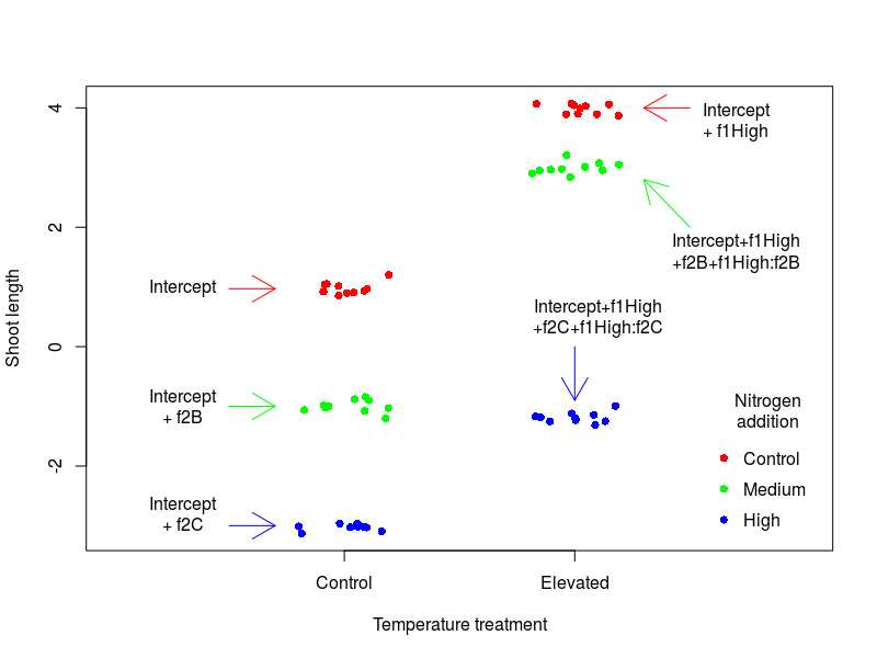
Let’s make an hypothetical examples: say we measured the shoot length (in cm) of some plant species under two different treatments: a temperature treatment with 2 levels (Control and Elevated temperature) and a nutrient treatment with three levels of nitrogen (Control, Medium, High nitrogen concentration). Following the recommendation of our stats professor we made a fully-factorial design and aim at look at the effect of these two treatments and their interactions on the shoot length.

#interpreting interaction coefficients from lm
#first case two categorical variables
set.seed(12)
f1<-gl(n=2,k=30,labels=c("Low","High"))
f2<-as.factor(rep(c("A","B","C"),times=20))
modmat<-model.matrix(~f1*f2,data.frame(f1=f1,f2=f2))
coeff<-c(1,3,-2,-4,1,-1.2)
y<-rnorm(n=60,mean=modmat%*%coeff,sd=0.1)
dat<-data.frame(y=y,f1=f1,f2=f2) summary(lm(y~f1*f2)) #output #Call: #lm(formula = y ~ f1 * f2) #Residuals: #      Min        1Q    Median        3Q       Max  #-0.199479 -0.063752 -0.001089  0.058162  0.222229  #Coefficients: #            Estimate Std. Error t value Pr(>|t|)    
#(Intercept)  0.97849    0.02865   34.15   <2e-16 ***
#f1High       3.00306    0.04052   74.11   <2e-16 ***
#f2B         -1.97878    0.04052  -48.83   <2e-16 ***
#f2C         -4.00206    0.04052  -98.77   <2e-16 ***
#f1High:f2B   0.98924    0.05731   17.26   <2e-16 ***
#f1High:f2C  -1.16620    0.05731  -20.35   <2e-16 ***
#---
#Signif. codes:  0 ‘***’ 0.001 ‘**’ 0.01 ‘*’ 0.05 ‘.’ 0.1 ‘ ’ 1
#
#Residual standard error: 0.09061 on 54 degrees of freedom
#Multiple R-squared:  0.9988,    Adjusted R-squared:  0.9987 
#F-statistic:  8785 on 5 and 54 DF,  p-value: < 2.2e-16

Let’s go through each coefficient:

• (Intercept): plant shoots are predicted to have a length of 0.98cm under control temperature and nitrogen conditions, this is our baseline.
• f1High: plant shoots grow 3cm bigger under elevated temperature and control nitrogen conditions compared to the baseline
• f2B: plant shoots grow ~2cm smaller under medium nitrogen and control temperature condition compared to the baseline
• f2C: plant shoots grow 4cm smaller under high nitrogen and control temperature condition compared to the baseline
• f1High:f2B : effect of medium nitrogen condition in plant shoots under elevated temperature increase by approx. 1 compared to the effect of medium nitrogen condition under control temperature conditions. In other words, when the effect of adding medium nitrogen was to decrease plant shoots length by ~2cm in control temperature condition, in elevated temperature conditions adding medium level of nitrogen lead to shoot length of 0.97 -1.97 + 3 + 0.98 = 3 on shoot length.
• f1High: f2C : same as above for high nitrogen condition.

The best way to grasp what these means is still to make a quick graph:

Not as easy to understand as one would thought …

Interaction between one continuous and one categorical variables

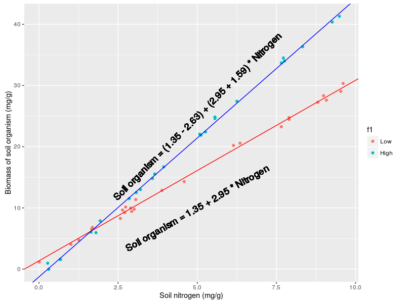
Say that we are weighting soil organisms in a field experiment where we added a temperature treatment with two levels (Control, Elevated) and we measured the soil nitrogen concentration (continuous variable measured in say mg per gram of soil), we would like to see the effects of the nitrogen concentration and its interaction with temperature on the biomass of soil organisms.

#second case one categorical and one continuous variable
x<-runif(50,0,10)
f1<-gl(n=2,k=25,labels=c("Low","High"))
modmat<-model.matrix(~x*f1,data.frame(f1=f1,x=x))
coeff<-c(1,3,-2,1.5)
y<-rnorm(n=50,mean=modmat%*%coeff,sd=0.5)
dat<-data.frame(y=y,f1=f1,x=x) summary(lm(y~x*f1)) #ouput #Call: #lm(formula = y ~ x * f1) # #Residuals: #    Min      1Q  Median      3Q     Max  #-0.9627 -0.2945 -0.1238  0.3386  0.9835  #Coefficients: #            Estimate Std. Error t value Pr(>|t|)    
#(Intercept)  1.35817    0.17959   7.563 1.31e-09 ***
#x            2.95059    0.03187  92.577  < 2e-16 ***
#f1High      -2.63301    0.25544 -10.308 1.54e-13 ***
#x:f1High     1.59598    0.04713  33.867  < 2e-16 ***
#---
#Signif. codes:  0 ‘***’ 0.001 ‘**’ 0.01 ‘*’ 0.05 ‘.’ 0.1 ‘ ’ 1

#Residual standard error: 0.4842 on 46 degrees of freedom
#Multiple R-squared:  0.9983,    Adjusted R-squared:  0.9981 
#F-statistic:  8792 on 3 and 46 DF,  p-value: < 2.2e-16

Again let’s go through the coefficients:

• (Intercept): Under control temperature condition and with a nitrogen concentration of 0 mg/g, soil organism biomass is 1.36 mg/g
• x: Adding 1mg/g of nitrogen increase soil organism biomass by 2.95 mg/g in control temperature conditions
• f1High: Under elevated temperature condition and for a nitrogen concentration of 0 mg/g soil organism biomass is 2.63 mg/g lower compared to control temperature condition
• x:f1High : the effect of soil nitrogen on soil organism biomass is higher by 1.59 under elevated temperature condition compared to control condition. In other words the slope between soil nitrogen and soil organism biomass is 2.95 + 1.59 = 4.54 in elevated temperature condition.

And a graph to grasp:

Interaction between two continuous variables

Now for the last possible case imagine that we wanted to compare our experimental results to what is happening in the “real” world. We went happily outside measured air temperature at the soil surface and collected soil samples from which we got soil nitrogen concentration (in mg per g of soil) and soil organism biomass (in mg per g of soil). Again we build a linear model to test the effect of temperature and nitrogen plus their interaction.

# third case interaction between two continuous variables
dat <- data.frame(nitrogen = runif(50, 0, 10), 
                  temperature= rnorm(50, 10, 3));
modmat <- model.matrix(~ nitrogen * temperature, dat);
coeff <- c(1, 2, -1, 1.5);
dat$soil <- rnorm(50, mean = modmat %*% coeff, sd = 0.5);

#fit a model
m <- lm(soil ~ nitrogen * temperature, dat);
summary(m)

Call:
lm(formula = soil ~ nitrogen * temperature, data = dat)

Residuals:
Min 1Q Median 3Q Max
-0.78742 -0.21694 0.00031 0.26940 0.92838

Coefficients:
Estimate Std. Error t value Pr(>|t|)
(Intercept) 1.541509 0.516898 2.982 0.00456 **
nitrogen 1.930706 0.083030 23.253 < 2e-16 ***
temperature -1.046353 0.050237 -20.828 < 2e-16 ***
nitrogen:temperature 1.505170 0.008279 181.815 < 2e-16 ***
---
Signif. codes: 0 ‘***’ 0.001 ‘**’ 0.01 ‘*’ 0.05 ‘.’ 0.1 ‘ ’ 1

Residual standard error: 0.4326 on 46 degrees of freedom
Multiple R-squared: 0.9999, Adjusted R-squared: 0.9999
F-statistic: 2.368e+05 on 3 and 46 DF, p-value: < 2.2e-16

The coefficient means:

• (Intercept): at 0°C and with nitrogen concentration of 0 mg/g, soil organism biomass is 0.96 mg/g
• nitrogen: increasing nitrogen concentration by 1 mg/g at a temperature of 0°C increase soil organism biomass by 1.93 mg/g
• temperature: increasing temperature by 1°C at a nitrogen concentration of 0 mg/g reduce the soil organism biomass by 1 mg/g
• nitrogen:temperature : (sit down and breath deeply) the effect of nitrogen on soil organism biomass increase by 1.50 for every unit increase in temperature. For example at a temperature of 0°C the slope between soil organism biomass and nitrogen is 1.93, at a temperature of 1°C this slope becomes: 1.93 + 1.50 * 1 = 3.43. This also works the other way round (ie effect of temperature on soil organism biomass become more positive as nitrogen concentration increase).

And a final graph:

new_d <- expand.grid(nitrogen=0:10,temperature=c(3.55,10,16))
new_d$Pred <- predict(m,new_d)

ggplot(dat,aes(x=nitrogen,y=soil,color=temperature))+
 geom_point()+
 geom_line(data=new_d,aes(group=temperature)) +
 scale_color_continuous(low="green",high="red") +
 geom_text(aes(x=5,y=20,label="Slope: (1.93 + 1.50 * 3.55) * nitrogen"),color="green",angle=13,family="Arial") +
 geom_text(aes(x=5,y=65,label="Slope: (1.93 + 1.50 * 10) * nitrogen"),color="brown",angle=30,family="Arial") +
 geom_text(aes(x=5,y=130,label="Slope: (1.93 + 1.50 * 16) * nitrogen"),color="red",angle=45,family="Arial")

 

 

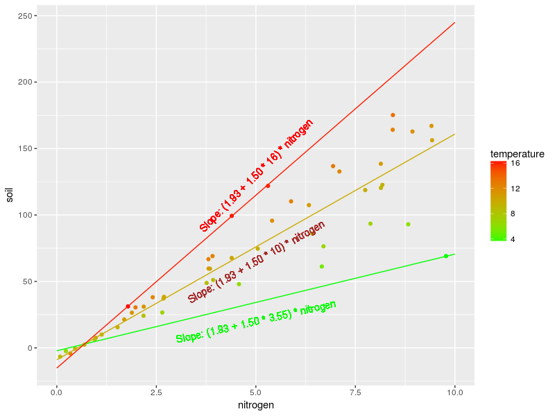
In this graph we drew the regression line of the relation between soil organism and soil nitrogen at three different temperature: at 3.55, 10 and 16°C. The text represent the slopes between soil organism and nitrogen and these different temperature. Note that you need to add the intercept plus the main effect of temperature to get the predicted value. For instance at nitrogen 5 mg/g and temperature 10°C we have:

soil organism = 1.54 – 1.04 * 10 + (1.93 + 1.50 * 10) * 5 = 75.79

So next time you want to fit 5-way interactions try to remember that already understanding two-way interaction need some thinking …

Happy coding.