UPDATED: Thanks to Ben and Florian comments I’ve updated the first part of the post
A very brief post at the end of the field season on two little “details” that are annoying me in paper/analysis that I see being done (sometimes) around me.
The first one concern mixed effect models where the models built in the contain a grouping factor (say month or season) that is fitted as both a fixed effect term and as a random effect term (on the right side of the | in lme4 model synthax). I don’t really understand why anyone would want to do this and instead of spending time writing equations let’s just make a simple simulation example and see what are the consequences of doing this:
library(lme4)
set.seed(20150830)
#an example of a situation measuring plant biomass on four different month along a gradient of temperature
data<-data.frame(temp=runif(100,-2,2),month=gl(n=4,k=25))
modmat<-model.matrix(~temp+month,data)
#the coefficient
eff<-c(1,2,0.5,1.2,-0.9)
data$biom<-rnorm(100,modmat%*%eff,1)
#the simulated coefficient for Months are 0.5, 1.2 -0.9
#a simple lm
m_fixed<-lm(biom~temp+month,data)
coef(m_fixed) #not too bad
## (Intercept)        temp      month2      month3      month4
##   0.9567796   2.0654349   0.4307483   1.2649599  -0.8925088

#a lmm with month ONLY as random term
m_rand<-lmer(biom~temp+(1|month),data)
fixef(m_rand)

## (Intercept)        temp
##    1.157095    2.063714

ranef(m_rand)

## $month
##   (Intercept)
## 1  -0.1916665
## 2   0.2197100
## 3   1.0131908
## 4  -1.0412343

VarCorr(m_rand) #the estimated sd for the month coeff

##  Groups   Name        Std.Dev.
##  month    (Intercept) 0.87720
##  Residual             0.98016

sd(c(0,0.5,1.2,-0.9)) #the simulated one, not too bad!

## [1] 0.8831761

#now a lmm with month as both fixed and random term
m_fixedrand<-lmer(biom~temp+month+(1|month),data) fixef(m_fixedrand) ## (Intercept) temp month2 month3 month4 ## 0.9567796 2.0654349 0.4307483 1.2649599 -0.8925088 ranef(m_fixedrand) #very, VERY small ## $month ## (Intercept) ## 1 0.000000e+00 ## 2 1.118685e-15 ## 3 -9.588729e-16 ## 4 5.193895e-16 VarCorr(m_fixedrand) ## Groups Name Std.Dev. ## month (Intercept) 0.40397 ## Residual 0.98018 #how does it affect the estimation of the fixed effect coefficient? summary(m_fixed)$coefficients ## Estimate Std. Error t value Pr(>|t|)
## (Intercept)  0.9567796  0.2039313  4.691676 9.080522e-06
## temp         2.0654349  0.1048368 19.701440 2.549792e-35
## month2       0.4307483  0.2862849  1.504614 1.357408e-01
## month3       1.2649599  0.2772677  4.562233 1.511379e-05
## month4      -0.8925088  0.2789932 -3.199035 1.874375e-03

summary(m_fixedrand)$coefficients

##               Estimate Std. Error    t value
## (Intercept)  0.9567796  0.4525224  2.1143256
## temp         2.0654349  0.1048368 19.7014396
## month2       0.4307483  0.6390118  0.6740851
## month3       1.2649599  0.6350232  1.9919901
## month4      -0.8925088  0.6357784 -1.4038048

#the numeric response is not affected but the standard error around the intercept and the month coefficient is doubled, this makes it less likely that a significant p-value will be given for these effect ie higher chance to infer that there is no month effect when there is some

#and what if we simulate data as is supposed by the model, ie a fixed effect of month and on top of it we add a random component
rnd.eff<-rnorm(4,0,1.2)
mus<-modmat%*%eff+rnd.eff[data$month]
data$biom2<-rnorm(100,mus,1)
#an lmm model
m_fixedrand2<-lmer(biom2~temp+month+(1|month),data)
fixef(m_fixedrand2) #weird coeff values for the fixed effect for month

## (Intercept)        temp      month2      month3      month4
##   -2.064083    2.141428    1.644968    4.590429    3.064715

c(0,eff[3:5])+rnd.eff #if we look at the intervals between the intercept and the different levels we can realize that the fixed effect part of the model sucked in the added random part

## [1] -2.66714133 -1.26677658  1.47977624  0.02506236

VarCorr(m_fixedrand2)

##  Groups   Name        Std.Dev.
##  month    (Intercept) 0.74327
##  Residual             0.93435

ranef(m_fixedrand2) #again very VERY small

## $month
##     (Intercept)
## 1  1.378195e-15
## 2  7.386264e-15
## 3 -2.118975e-14
## 4 -7.752347e-15

#so this is basically not working it does not make sense to have a grouping factor as both a fixed effect terms and a random term (ie on the right-hand side of the |)
Take-home message don’t put a grouping factor as both a fixed and random term effect in your mixed effect model. lmer is not able to separate between the fixed and random part of the effect (and I don’t know how it could be done) and basically gives everything to the fixed effect leaving very small random effects. The issue is abit pernicious because if you would only look at the standard deviation of the random term from the merMod summary output you could not have guessed that something is wrong. You need to actually look at the random effects to realize that they are incredibely small. So beware when building complex models with many fixed and random terms to always check the estimated random effects.
Now this is only true for factorial variables, if you have a continuous variable (say year) that affect your response through both a long-term trend but also present some between-level (between year) variation, it actually makes sense (provided you have enough data point) to fit a model with this variable as both a fixed and random term. Let’s look into this:
#an example of a situation measuring plant biomass on 10 different year along a gradient of temperature
set.seed(10)
data<-data.frame(temp=runif(100,-2,2),year=rep(1:10,each=10))
modmat<-model.matrix(~temp+year,data)
#the coefficient
eff<-c(1,2,-1.5)
rnd_eff<-rnorm(10,0,0.5)
data$y<-rnorm(100,modmat%*%eff+rnd_eff[data$year],1)
#a simple lm
m_fixed<-lm(y~temp+year,data)
summary(m_fixed)

Call:
lm(formula = y ~ temp + year, data = data)

Residuals:
Min       1Q   Median       3Q      Max
-2.27455 -0.83566 -0.03557  0.92881  2.74613

Coefficients:
Estimate Std. Error t value Pr(>|t|)
(Intercept)  1.41802    0.25085   5.653 1.59e-07 ***
temp         2.11359    0.11230  18.820  < 2e-16 ***
year        -1.54711    0.04036 -38.336  < 2e-16 ***
---
Signif. codes:  0 ‘***’ 0.001 ‘**’ 0.01 ‘*’ 0.05 ‘.’ 0.1 ‘ ’ 1

Residual standard error: 1.159 on 97 degrees of freedom
Multiple R-squared:  0.9508,    Adjusted R-squared:  0.9498
F-statistic: 937.1 on 2 and 97 DF,  p-value: < 2.2e-16
coef(m_fixed) #not too bad

(Intercept)        temp        year
1.418019    2.113591   -1.547111
#a lmm
m_rand<-lmer(y~temp+year+(1|factor(year)),data)
summary(m_rand)

Linear mixed model fit by REML ['lmerMod']
Formula: y ~ temp + year + (1 | factor(year))
Data: data

REML criterion at convergence: 304.8

Scaled residuals:
Min      1Q  Median      3Q     Max
-2.0194 -0.7775  0.1780  0.6733  1.9903

Random effects:
Groups       Name        Variance Std.Dev.
factor(year) (Intercept) 0.425    0.6519
Residual                 1.004    1.0019
Number of obs: 100, groups:  factor(year), 10

Fixed effects:
Estimate Std. Error t value
(Intercept)  1.40266    0.49539   2.831
temp         2.01298    0.10191  19.752
year        -1.54832    0.07981 -19.400

Correlation of Fixed Effects:
(Intr) temp
temp  0.031
year -0.885  0.015
fixef(m_rand) #very close to the lm estimation

(Intercept)        temp        year
1.402660    2.012976   -1.548319
plot(rnd_eff,ranef(m_rand)[[1]][,1])
abline(0,1) #not too bad
VarCorr(m_rand) #the estimated sd for the within-year variation

Groups       Name        Std.Dev.
factor(year) (Intercept) 0.65191
Residual                 1.00189
Interestingly we see in this case that the standard error (and the related t-value) of the intercept and year slope are twice as big (small for the t-values) in the LMM compared to the LM. This means that not taking into account between-year random variation leads us to over-estimate the precision of the long-term temporal trend (we might conclude that there are significant effect when there are a lot of noise not taken into account). I still don’t fully grasp how this work, but thanks to the commenter for pointing this out.
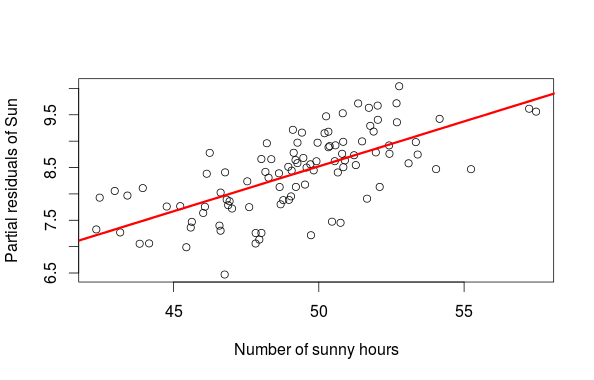
The second issue is maybe a bit older but I saw it appear in a recent paper (which is a cool one excpet for this stats detail). After fitting a model with several predictors one wants to plot their effects on the response, some people use partial residuals plot to do this (wiki). The issue with these plots is that when two variables have a high covariance the partial residual plot will tend to be over-optimistic concerning the effect of variable X on Y (ie the plot will look much nice than it should be). Again let’s do a little simulation on this:
library(MASS)
set.seed(20150830)
#say we measure plant biomass in relation with measured temperature and number of sunny hours say per week
#the variance-covariance matrix between temperature and sunny hours
sig<-matrix(c(2,0.7,0.7,10),ncol=2,byrow=TRUE)
#simulate some data
xs<-mvrnorm(100,c(5,50),sig)
data<-data.frame(temp=xs[,1],sun=xs[,2])
modmat<-model.matrix(~temp+sun,data)
eff<-c(1,2,0.2)
data$biom<-rnorm(100,modmat%*%eff,0.7)

m<-lm(biom~temp+sun,data)
sun_new<-data.frame(sun=seq(40,65,length=20),temp=mean(data$temp))
#partial residual plot of sun
sun_res<-resid(m)+coef(m)[3]*data$sun
plot(data$sun,sun_res,xlab="Number of sunny hours",ylab="Partial residuals of Sun")
lines(sun_new$sun,coef(m)[3]*sun_new$sun,lwd=3,col="red")
#plot of sun effect while controlling for temp
pred_sun<-predict(m,newdata=sun_new)
plot(biom~sun,data,xlab="Number of sunny hours",ylab="Plant biomass")
lines(sun_new$sun,pred_sun,lwd=3,col="red")
#same stuff for temp
temp_new<-data.frame(temp=seq(1,9,length=20),sun=mean(data$sun))
pred_temp<-predict(m,newdata=temp_new)
plot(biom~temp,data,xlab="Temperature",ylab="Plant biomass")
lines(temp_new$temp,pred_temp,lwd=3,col="red")
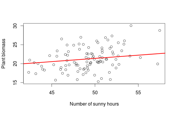
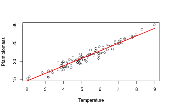
The first graph is a partial residual plot, from this graph alone we would be tempted to say that the number of hour with sun has a large influence on the biomass. This conclusion is biased by the fact that the number of sunny hours covary with temperature and temperature has a large influence on plant biomass. So who is more important temperature or sun? The way to resolve this is to plot the actual observation and to add a fitted regression line from a new dataset (sun_new in the example) where one variable is allowed to vary while all others are fixed to their means. This way we see how an increase in the number of sunny hour at an average temperature affect the biomass (the second figure). The final graph is then showing the effect of temperature while controlling for the effect of the number of sunny hours.
Happy modelling!


Regarding inclusion of the same variable as a fixed and as a random effect, this is a situation in which the assumption of independence of the fixed and the random part of the model is (very badly) violated. Generally, if such a violation occurs, the fixed effect will be overestimated and the random effect (variance) will be underestimated, see: Ebbes, P., Böckenholt, U. i Wedel, M. (2004). Regressor and random-effects dependencies in multilevel models. Statistica Neerlandica 58(2), 161-178.
Thanks a lot for your comments! I was not aware of this paper so thanks for sharing it.
Two thoughts: (1) I don’t know if there’s an easy way to detect this situation, but you could post an issue/your example at https://github.com/lme4/lme4/issues … (2) in the case where the covariate is *continuous* (numeric), but has repeated observations at each level (e.g. year 1, 2, 3, 4 …) it *can* make sense to use a model of the form response ~ … + covariate + (1|covariate) … — the fixed term is linear and the random term automatically treats the grouping variable as categorical.
Your second point is interesting, the fixed term would then represent the slope of the covariate effect (year) but what would the random effect coefficient represent in that case? The extra deviation of each individual level (years) from the overall trend? How can the model separate between what is explained by the overall trend in the covariate and random deviates from this trend using only the information provided by that one covariate? In my (limited) experience of such models fit to empirical data the random effects were all very small (ie 1e-16).
I agree with Ben – if the variable is categorical, it doesn’t make sense, so a warning would be good. If it is continuous as in year, however, it totally makes sense to have both, year is a typical case where you take out long-term trends and random variation between years at the same time (you should have enough observations of course).
I am proven wrong! I have been trying out as you said with a continuous random effect and lmer works pretty well, I still don’t know how the model is able to differentiate between what is long-term trend (the slope) and what is random between-year variation (random effect) … I am updating the post.
It works because the fixed continuous effect fits treats the variable as a number, while the random effect treats it as an unordered grouping factor only, so it won’t react to a trend.
Make sense, I wonder about how some results/interpretations in my field of reseach (Biodversity and Ecosystem Function) would hold if we would similar models but with species richness instead of year…
Not sure why one would use richness as a random effect – it would make sense to me to have the specific species mixture as random, and richness as fixed though
Well, to capture the overall trend of say plant species richness on plant biomass while controlling for random variation between richness levels. Conceptually I do find it very close to the example of year, again I might be wrong …
I think that Ben’s suggestion is rather tricky. Of course someone may want to control influence of some covariate in such a way, but we should ask a question, whether such a model allows for making reasonable inference. And I think it doesn’t. Such a specification obviously violates the assumption of independence between fixed and random part of the model. That means we may expect troubles… and it can be found with simulation studies, that in such a situation estimates of the fixed effect are biased upward and estimates of the random effect are (heavily) biased downward. Moreover specification proposed by Ben can be seen simply as a rough way to model nonlinearity. But I think it would be much better to make some efforts to model nonlinear effect of such a covariate in explicit manner, with set of fixed effects.
Thanks for this! If I understand things correctly seems like there is another case where including the same factor as both a fixed and random effect leads to valid model specification. That’s when it’s important to model the interaction between a fixed categorical effect and another, random categorical effect.
Ben Bolker hints at this on the FAQ page: https://bbolker.github.io/mixedmodels-misc/glmmFAQ.html#model-specification, and gives an excellent example here: https://stats.stackexchange.com/a/70607/171222, where he voices approval for the lmer specification y~fixed_factor+(1|fixed_factor:random_factor).