Interpreting random effects in linear mixed-effect models

Recently I had more and more trouble to find topics for stats-orientated posts, fortunately a recent question from a reader gave me the idea for this one.

In this post I will explain how to interpret the random effects from linear mixed-effect models fitted with lmer (package lme4). For more informations on these models you can browse through the couple of posts that I made on this topic (like here, here or here).

The Intuition

Random effects can be thought as being a special kind of interaction terms. For example imagine you measured several times the reaction time of 10 people, one could assume (i) that on average everyone has the same value or (ii) that every person has a specific average reaction time. In the second case one could fit a linear model with the following R formula:

Reaction ~ Subject

Mixed-effect models follow a similar intuition but, in this particular example, instead of fitting one average value per person, a mixed-effect model would estimate the amount of variation in the average reaction time between the person.

A simple example

Let’s go through some R code to see this reasoning in action:

#load libraries
library(lme4)
library(ggplot2)
library(reshape2)

#load example data
data("sleepstudy")

#a simple example
m_avg <- lmer(Reaction ~ 1 + (1|Subject),sleepstudy)

The model m_avg will estimate the average reaction time across all subjects but it will also allow the average reaction time to vary between the subject (see here for more infos on lme4 formula syntax). We can access the estimated deviation between each subject average reaction time and the overall average:

ranef(m_avg)

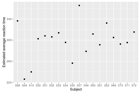
ranef returns the estimated deviation, if we are interested in the estimated average reaction time per subject we have to add the overall average to the deviations:

#to get the fitted average reaction time per subject
reaction_subject <- fixef(m_avg) + ranef(m_avg)$Subject
reaction_subject$Subject<-rownames(reaction_subject)
names(reaction_subject)[1]<-"Intercept"
reaction_subject <- reaction_subject[,c(2,1)]
#plot
ggplot(reaction_subject,aes(x=Subject,y=Intercept))+geom_point()

A very cool feature of mixed-effect models is that we can estimate the average reaction time of hypothetical new subjects using the estimated random effect standard deviation:

#This line create a dataframe for 18 hypothetical new subjects
#taking the estimated standard deviation reported in
#summary(m_avg)
new_subject <- data.frame(Subject = as.character(400:417),
  Intercept= fixef(m_avg)+rnorm(18,0,35.75),Status="Simulated")
reaction_subject$Status <- "Observed"
reaction_subject <- rbind(reaction_subject,new_subject)
#new plot
ggplot(reaction_subject,aes(x=Subject,y=Intercept,color=Status))+
  geom_point()+
  geom_hline(aes(yintercept = fixef(m_avg)[1],linewidth=1.5))

A more complex example

The second intuition to have is to realize that any single parameter in a model could vary between some grouping variables (i.e. the subjects in this example). For instance one could measure the reaction time of our different subject after depriving them from sleep for different duration. We could expect that the effect (the slope) of sleep deprivation on reaction time can be variable between the subject, each subject also varying in their average reaction time. In this case two parameters (the intercept and the slope of the deprivation effect) will be allowed to vary between the subject and one can plot the different fitted regression lines for each subject:

#fit the model
m_slp <- lmer(Reaction ~ Days + (Days | Subject), sleepstudy)
#the next line put all the estimated intercept and slope per
#subject into a dataframe
reaction_slp <- as.data.frame(t(apply(ranef(m_slp)$Subject,
  1,function(x) fixef(m_slp) + x)))
#to get the predicted regression lines we need one further
#step, writing the linear equation: Intercept + Slope*Days
#with different coefficient for each subject
pred_slp <- melt(apply(reaction_slp,1,function(x) x[1] + x[2]*0:9),
  value.name = "Reaction")
#some re-formatting for the plot
names(pred_slp)[1:2] <- c("Days","Subject")
pred_slp$Days <- pred_slp$Days - 1
pred_slp$Subject <- as.factor(pred_slp$Subject)

#plot with actual data
ggplot(pred_slp,aes(x=Days,y=Reaction,color=Subject))+
  geom_line()+
  geom_point(data=sleepstudy,aes(x=Days,y=Reaction))+
  facet_wrap(~Subject,nrow=3)

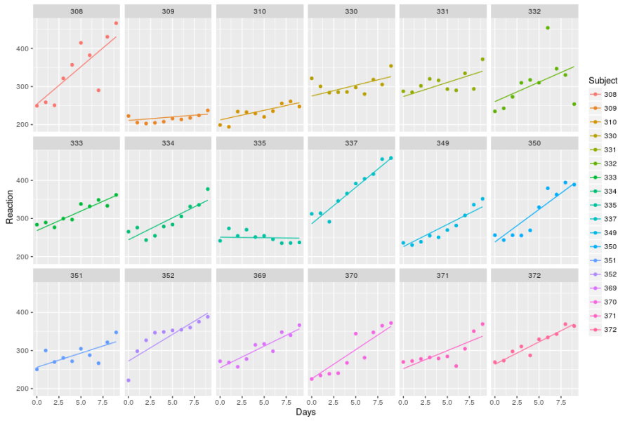
In this graph we clearly see that while some subjects’ reaction time is heavily affected by sleep deprivation (n° 308) others are little affected (n°335). Even more interesting is the fact that the relationship is linear for some (n°333) while clearly non-linear for others (n°352).

Again we could simulate the response for new subjects sampling intercept and slope coefficients from a normal distribution with the estimated standard deviation reported in the summary of the model.

After reading this post readers may wonder how to choose, then, between fitting the variation of an effect as a classical interaction or as a random-effect, if you are in this case I point you towards this post and the lme4 FAQ webpage.

Happy coding and don’t hesitate to ask questions as they may turn into posts!